13일차 [ 데이터분석: Pandas ]

개발공부/SK Networks Family AI bootcamp 강의노트

13일차 [ 데이터분석: Pandas ]

HyunJung_Jo 2025. 1. 31. 17:22

가성비 최고로 검증된 딥시크의 충격.... 공부 좀 해야겠다.

독립변수,종속변수 (cause and effect)

상관관계 (증감,우상향,우하향 등)
상관관계 인과관계
상관관계에서 인과관계가 되는지 가설을 세우고, 참이 되면 인과관계가 성립이 된다.
p값<0.05, 귀무가설(null hypothesis) 기 (비료양은 수확량에 영향 안 준다)

Colab

https://drive.google.com/drive/folders/1sVzLoGwO_NmRg1uFu9yTwZqfh7ggDpNt

Google Drive: 로그인

이메일 또는 휴대전화

accounts.google.com

런타임 유형 변경 > cpu, gpu 중 선택 가능

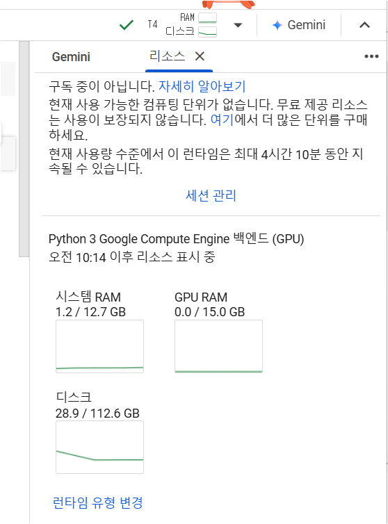
ctrl+s 로 필히 저장
세션관리 > 종료 눌러야 비용청구가 안된다.

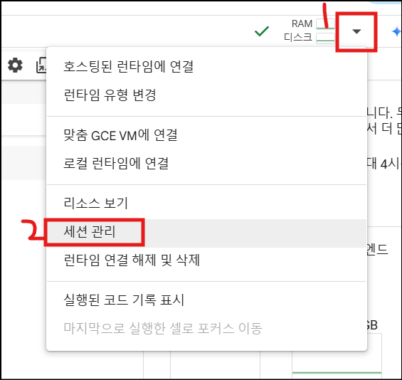
현재 오픈한 코랩 페이지에서는 '런타임 연결 해제 및 삭제' 눌러서 관리

Pandas

Vector,1차원 데이터,Series

cell 내에서 lib 설치 : !pip install pandas
데이터 타입 최적화로 비용 줄이기 (np.in8, float64->int8)

import pandas as pd
data = {
    'a':1.0, 'b':2.0, 'c':3.0
}

series = pd.Series(data, index=['a','b','c'])
# dtype: float64

#######################
import numpy as np
pd.Series(data=data,dtype=np.int8,index=['a','b','c'])
# dtype:int8

가우시안 정규분포

pd.Series(data=np.random.randn(5))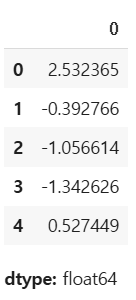

slicing, index

vector = pd.Series(data=np.random.randn(5),name='randn')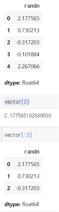

통계 수치 (평균,중위값,최대값)

vector.median() # 중위값
# 중위값보다 큰 데이터를 조회
vector[vector > vector.median()]

vector.mean() # 평균값
# 평균보다 큰 데이터 조회
vector[vector > vector.mean()]

vector.max() #최대값
vector[vector==vector.max()]

데이터 수정

vector[0]=3.141592
vector[3:]=np.random.randn(2)

사칙연산

vector + vector, v-v, v/v, v*v 다 가능

절대값: vector.abs()

데이터 형 변환

list(vector)

list(vector)
# [3.141592,
 # 0.7302129917333388,
 # -0.3172025162359212,
 # 0.12595782948126646,
 # -0.5736458018616561]
 
 list(vector.index)
 [0, 1, 2, 3, 4]
 
 list(vector.items())
 [(0, 3.141592),
 (1, 0.7302129917333388),
 (2, -0.3172025162359212),
 (3, 0.12595782948126646),
 (4, -0.5736458018616561)]

Matrix, 2차원 데이터, DataFrame

data = {
    'Jenny':pd.Series([90,80,95]),
    'James':pd.Series([80,90,100])
}
df = pd.DataFrame(data)

list(df.index)
[0, 1, 2]

df.columns
Index(['Jenny', 'James'], dtype='object')

df.shape (index 크기 , column 크기)
(3,2)

데이터 형 변환, to_dict

df.to_dict()
{'Jenny': {0: 90, 1: 80, 2: 95}, 'James': {0: 80, 1: 90, 2: 100}}

df.to_dict('series')
{'Jenny': 0    90
 1    80
 2    95
 Name: Jenny, dtype: int64,
 'James': 0     80
 1     90
 2    100
 Name: James, dtype: int64}
 
type(df.to_dict('series')['Jenny']) # series

df.to_dict('records') # 웹 개발에서 많이 씀
[{'Jenny': 90, 'James': 80},
 {'Jenny': 80, 'James': 90},
 {'Jenny': 95, 'James': 100}]
 
 df.to_json(orient='records')
 [{"Jenny":90,"James":80},{"Jenny":80,"James":90},{"Jenny":95,"James":100}]
 
 print(df.to_csv())
 ,Jenny,James
0,90,80
1,80,90
2,95,100

records
- records는 데이터베이스, 데이터 프레임, 그리고 다양한 데이터 구조에서 개별 데이터 항목이나 엔트리를 나타내는 개념입니다. 이 용어는 주로 다음과 같은 맥락에서 사용됩니다.
  
  데이터베이스에서는 테이블의 각각의 행(row)을 "레코드"라고 부릅니다. 예를 들어, 고객 정보가 담긴 테이블에서 각 고객의 정보가 하나의 레코드로 나타납니다.
  
  레코드는 여러 필드(field)로 구성되며, 각 필드는 해당 레코드에 대한 데이터를 포함합니다.

데이터 수정,삭제

df['Mari']=df['Jenny']+df['James']
df['is_over_90']=df['Jenny']>90df

del df['is_over_90'] # df 조회 안됨
 df.pop('Mari') # df 조회 됨

slice / index

col명, iloc, loc

# col 기준=================
df['Jenny'][2]
95

df['Jenny'][2:]


# row 기준/ index location==
df.iloc[2]

2
Jenny	95
James	100

df.iloc[2:]

# index(row), col  으로 slicing 
df.iloc[2:,:] # index(row), col

# loc
df.loc[:,'Jenny'] # Jenny라는 col명으로 접근

통계 데이터

import seaborn as sns
iris = sns.load_dataset('iris')

iris.shape
(150, 5)


iris.info()
<class 'pandas.core.frame.DataFrame'>
RangeIndex: 150 entries, 0 to 149
Data columns (total 5 columns):
 #   Column        Non-Null Count  Dtype  
---  ------        --------------  -----  
 0   sepal_length  150 non-null    float64
 1   sepal_width   150 non-null    float64
 2   petal_length  150 non-null    float64
 3   petal_width   150 non-null    float64
 4   species       150 non-null    object 
dtypes: float64(4), object(1)
memory usage: 6.0+ KB


iris.describe()
sepal_length	sepal_width	petal_length	petal_width
count	150.000000	150.000000	150.000000	150.000000
mean	5.843333	3.057333	3.758000	1.199333
std	0.828066	0.435866	1.765298	0.762238
min	4.300000	2.000000	1.000000	0.100000
25%	5.100000	2.800000	1.600000	0.300000
50%	5.800000	3.000000	4.350000	1.300000
75%	6.400000	3.300000	5.100000	1.800000
max	7.900000	4.400000	6.900000	2.500000


iris['species'].describe()
species
count	150
unique	3
top	setosa
freq	50

dtype: object
>> 3개의 종, 가장 많은 건 setosa, 가장 빈번했던 건 50개였음.

iris[iris['sepal_length']>5.0]['sepal_length'].min() # 스칼라 0차원
       # matrix               # vector       # scalar
# 5.1

iris[iris['sepal_length']>5.0].iloc[:,:-1].median(axis=0) 
# row 데이터에 대한 medium 값을 뽑는다.(column,)


0
sepal_length	6.1
sepal_width	3.0
petal_length	4.7
petal_width	1.5

dtype: float64

iris[iris['sepal_length']>5.0].iloc[:,:-1].median(axis=1)
# column 데이터에 대한 medium값을 뽑는다. (row,) 


0
0	2.45
5	2.80
10	2.60
14	2.60
15	2.95
...	...
145	4.10
146	3.75
147	4.10
148	4.40
149	4.05
118 rows × 1 columns


dtype: float64

iris[iris['sepal_length']>5.0].iloc[:,:-1].median(axis=0).median() # scalar

cond1 = iris['sepal_length']>5.0
cond2 = iris['sepal_width']>3.0
iris[cond1 & cond2].head()
# True & True 아니면 모두 False, 교집합; AND


sepal_length	sepal_width	petal_length	petal_width	species
0	5.1	3.5	1.4	0.2	setosa
5	5.4	3.9	1.7	0.4	setosa
10	5.4	3.7	1.5	0.2	setosa
14	5.8	4.0	1.2	0.2	setosa
15	5.7	4.4	1.5	0.4	setosa

iris[cond1 & cond2].shape
(47,5)

# ====================================
cond1 = iris['sepal_length']>5.0
cond2 = iris['sepal_width']>3.0
iris[cond1 | cond2].head()
# False | False 아니면 모두 True, 합집합; OR
iris[cond1 | cond2].shape
(138, 5)

# ====================================
iris[~cond].shape
(128,5) # 차집합,NOT

import numpy as np
iris.select_dtypes(include=[np.number,object]).head()

iris.select_dtypes(include=['float']).head()

iris.select_dtypes(exclude=np.number).head()

Pandas 심화

import seaborn as sns
df = sns.load_dataset('titanic')
df.shape

df.info() # features는 독립변수 및 종속변수
# survived, 종속변수  / 그 외엔 독립변수 
# shape, dtype, feature name, 결측치(null) 유무, 사용하는 메모리 양
<class 'pandas.core.frame.DataFrame'>
RangeIndex: 891 entries, 0 to 890
Data columns (total 15 columns):
 #   Column       Non-Null Count  Dtype   
---  ------       --------------  -----   
 0   survived     891 non-null    int64   
 1   pclass       891 non-null    int64   
 2   sex          891 non-null    object  
 3   age          714 non-null    float64 
 4   sibsp        891 non-null    int64   
 5   parch        891 non-null    int64   
 6   fare         891 non-null    float64 
 7   embarked     889 non-null    object  
 8   class        891 non-null    category
 9   who          891 non-null    object  
 10  adult_male   891 non-null    bool    
 11  deck         203 non-null    category
 12  embark_town  889 non-null    object  
 13  alive        891 non-null    object  
 14  alone        891 non-null    bool    
dtypes: bool(2), category(2), float64(2), int64(4), object(5)
memory usage: 80.7+ KB

df.select_dtypes(exclude=['number']).describe()

sex	embarked	class	who	adult_male	deck	embark_town	alive	alone
count	891	889	891	891	891	203	889	891	891
unique	2	3	3	3	2	7	3	2	2
top	male	S	Third	man	True	C	Southampton	no	True
freq	577	644	491	537	537	59	644	549	537

# 결측치 =========================
df.isnull().sum(axis=0) # 컬럼별로 결측치 보기
	        0
survived	0
pclass	0
sex	0
age	177
sibsp	0
parch	0
fare	0
embarked	2
class	0
who	0
adult_male	0
deck	688
embark_town	2
alive	0
alone	0

# number ======================
dtype: int64
df_number = df.select_dtypes(include=['number'])
df_number.mean() # 그 외 min,max, median,sum 등 가능

# object ===============
df_object = df.select_dtypes(include=['object'])
df_object['sex'].value_counts()

count
sex	
male	577
female	314

dtype: int64

df_object['sex'].nunique() # 2
df_object['sex'].unique() # array(['male', 'female'], dtype=object)
# 성별로 봤을 때 가장 많은 것
df_object['sex'].value_counts().idxmax()

map() (1차원, series)

x = pd.Series(
    {
        'one':1,
        'two':2,
        'three':3
    }
)
x
# index:data 쌍으로 구성

y = pd.Series(
    {
        1:'a',
        2:'aa',
        3:'aaa'
    }
)

x.map(y)
# x value값을 y의 index에 적용
# y value를 x value값에 치환
	0
one	a
two	aa
three	aaa

## sex male, female -> 0,1
df['gender'] = df['sex'].map({'male': 0, 'female': 1})
df['sex'].map(lambda data:1 if data=='male' else 2).head()

apply() (2차원, df 조작)

df['new_age']=df['age'].apply(lambda data:data*10)

df['new_age']=df.apply(lambda data: data['age']*10 if data['sex']=='male' else data['age']*5,axis=1)
df[['sex','age','new_age']].head()

df.select_dtypes(include=['number']).apply(lambda data:data.mean(),axis=0)

def add_column(row):
  return row['age']+row['fare']
df['add_column'] = df.apply(add_column,axis=1)
df.head()

pivot table

df_tmp = df[['survived','age','fare','pclass','sex']]

pd.pivot_table(
    data = df_tmp,
    index = 'sex',# 분석시 사용 기준이 되는 data col
    columns = 'pclass', # 분석시 사용 기준되는 data col
    values = 'survived', # target col
    aggfunc =['mean','median']
)

mean	median
pclass	1	2	3	1	2	3
sex						
female	0.968085	0.921053	0.500000	1.0	1.0	0.5
male	0.368852	0.157407	0.135447	0.0	0.0	0.0

# =>pclass 숫자가 낮고 여자일 수록 살 확률이 높다.

pd.pivot_table(
    data = df_tmp,
    index = 'sex',# 분석시 사용 기준이 되는 data col
    columns = 'pclass', # 분석시 사용 기준되는 data col
    values = 'fare', # target col
    aggfunc =['mean','median']
)


mean	median
pclass	1	2	3	1	2	3
sex						
female	106.125798	21.970121	16.118810	82.66455	22.0	12.475
male	67.226127	19.741782	12.661633	41.26250	13.0	7.925

# => pclass가 낮고 여자일 수록 요금이 높다.

정제된 데이터를 줘야 인사이트를 얻고, 모델 학습하기도 좋다.

생각보다 판다스를 잘 정리해주셔서 공부하기 좋았다. 배부된 판다스 책을 어떻게 봐야할 지 조금 막막하지만, 이 강의자료라도 충분히 숙지해두면 좋을 것 같다.

https://github.com/good593/class_data_analysis/tree/main

GitHub - good593/class_data_analysis

Contribute to good593/class_data_analysis development by creating an account on GitHub.

github.com

'개발공부 > SK Networks Family AI bootcamp 강의노트' 카테고리의 다른 글

[플레이데이터 SK네트웍스 Family AI캠프 10기] 3주차 회고 (0)	2025.01.24
12일차 [ Web Crawling2 ] (0)	2025.01.22
토이 프로젝트 일정 (자동 코인 매매 봇) (0)	2025.01.21
11일차 [ Web crawling ] (1)	2025.01.21
11일차 [ streamlit ] (0)	2025.01.21

현재글13일차 [ 데이터분석: Pandas ]

끄적끄적 인생기

Today :
Yesterday :

끄적끄적 인생기

13일차 [ 데이터분석: Pandas ]

독립변수,종속변수 (cause and effect)

Colab

Pandas

Vector,1차원 데이터,Series

slicing, index

통계 수치 (평균,중위값,최대값)

데이터 수정

사칙연산

데이터 형 변환

Matrix, 2차원 데이터, DataFrame

데이터 형 변환, to_dict

데이터 수정,삭제

slice / index

통계 데이터

Pandas 심화

map() (1차원, series)

apply() (2차원, df 조작)

pivot table

'개발공부 > SK Networks Family AI bootcamp 강의노트' 카테고리의 다른 글

'개발공부/SK Networks Family AI bootcamp 강의노트'의 다른글

티스토리툴바

« 2025/02 »
일	월	화	수	목	금	토
						1
2	3	4	5	6	7	8
9	10	11	12	13	14	15
16	17	18	19	20	21	22
23	24	25	26	27	28

13일차 [ 데이터분석: Pandas ]

독립변수,종속변수 (cause and effect)

Colab

Pandas

Vector,1차원 데이터,Series

slicing, index

통계 수치 (평균,중위값,최대값)

데이터 수정

사칙연산

데이터 형 변환

Matrix, 2차원 데이터, DataFrame

데이터 형 변환, to_dict

데이터 수정,삭제

slice / index

통계 데이터

Pandas 심화

map() (1차원, series)

apply() (2차원, df 조작)

pivot table

'개발공부 > SK Networks Family AI bootcamp 강의노트' 카테고리의 다른 글

'개발공부/SK Networks Family AI bootcamp 강의노트'의 다른글

관련글

티스토리툴바